Training a Text-to-Image Model for $21K

249 samples · 2B Pyramid-JiT

Click any picture for full resolution and its prompt

Pressure testing the Pyramid-JiT (P-JiT)

For us, this $21K training run is a proof-of-concept along the way to our next video model. We were surprised by how good the results looked given the size of the model, so we thought we'd share it with the world as an experimental release.

If you haven't followed our work previously, we'd love to take a step back and introduce ourselves. We're a 2-person research lab training our own generative video models entirely from scratch. The ultimate ambition is creative tools that democratize access to animation. You can read more about that here.

Today, generative video models have two major flaws: they are too slow/expensive and they lack proper controls. Creativity is an iterative process. You make, you tweak, you get better. With this double whammy, video models (as they stand today) are effectively useless for storytelling.

When we set out to build Linum v3 earlier this year, the primary goal was to bring the cost envelope of inference down significantly. If our model is fast and cheap, it's the first step (of many) towards useful creative tools.

We've written extensively about the steps we've taken in this direction, but here's the long story short:

The bottleneck for training and inference for video is attention, O(n²). If we can compress more aggressively, we'll reduce the context window for attention, slashing the cost of training and inference.
Typically, compression is handled by a separate specialized model like a Variational Autoencoder, but that's not necessarily optimal. VAEs seem to have an empirical ceiling on the amount of compression they can achieve.There are other ways to get more compression, but they require substantial surgery to the traditional VAE (e.g. the 2B decoder in Minimax's H3). More importantly, improving the VAE on its task of reconstruction can produce worse generations in the downstream diffusion model.
If you get rid of the VAE altogether, you should be able to compress more aggressively and learn faster. Diffusion models are a more powerful family of generative models than VAEs. We should be able to use them to compress and generate at the same time. Instead of using another model's latent space, the diffusion model should learn a latent space purpose-built for its use case. In turn, we should be able to squeeze more juice out of this compression.

In our last blog, we iterated towards a new architecture that we called the Pyramid-JiT (P-JiT). It's a pixel-space model that converges in 11× fewer samples than Linum v2 with 4× more aggressive token reduction (i.e., we represent a 512² image in the same number of tokens we used to represent a 256² image).Linum v2 is a fairly standard Wan VAE + DiT diffusion model. Linum v2 used a 16×16 token reduction like most models (e.g. FLUX-2). P-JiT enables 32×32 token reduction. This implies a 4× reduction in attention context-window.

For the details on how we got there, we'd recommend you take a look at our previous blogs on JiT-DDT and P-JiT. But at a high level, we found a noise schedule for pixel-space models that helps the models better learn fine-grained detail. And, we added readouts along the trunk of the DiT.

Adjacent work in REPA, RAE-v2, and Self-Flow all point to weak gradients in the early blocks of the DiT. By operating in pixel space, every block of our DiT is quite literally predicting a version of the final image, so we can boost gradient signal earlier in the network by predicting low-resolution versions of the final image. This helps accelerate convergence.

The architecture did well in our initial experiments, but we wanted to see how it performed when we trained it for longer (i.e., ~600M samples instead of 50–100M samples).For context, generative video models pretty much always start as generative image models. You have to learn nouns (people, places, things) before you can learn verbs (actions, movement). It's a pressure test of sorts along the way towards larger models (and video).

Training Regime

sizes read 512² stage / 1024² stage · flower = an illustrative target2.18B params at sampling · purple heads are training-only and add ~0.24B, for ~2.42B in training

Text and image each pass through two single-modality "refiner" DiT blocks, then merge into one stream of 22 identical DiT blocks. The text representation comes from a frozen Qwen3.5-4B model, which we read at layers 7, 15 and 27 (its three full-attention layers). We concatenate and project these representations into the text refiner. The image is split into 32×32 patches and compressed into a 1024-dimensional space, before being projected up into the image refiner blocks.This is a 3:1 compression rate. A 32×32 patch with RGB values is a 32×32×3 = 3,072 representation, which gets projected into 1024 dimensions.

At block 5, we have a 2-layer PixelREPA readout that aligns the model's latent space to DINOv3-L.We mask 20% of the tokens in our hidden state and push it through a 2-layer transformer to predict DINOv3-L's feature representation of the same image. We have two linear readout heads along the trunk after blocks 10 and 16. As discussed earlier, these predict the clean image at a quarter and half resolution, respectively. The total loss is given by MSE at the readouts, PixelREPA cosine-distance, MSE at the final output head, and perceptual losses on the full resolution image (LPIPS and P-DINO).

blue = AdaLN · s scales the input before attention/FFN, g gates its residual writehidden size 2,944 · 23 heads × 128 · FFN inner width 5,376 in the trunk, 2,816 in the refiners

Every DiT block is conditioned on the timestep through a low-rank AdaLN, following Z-Image. The timestep embedding goes through one down-projection to 256-dim.The image refiner and trunk share one down-projection; the text refiner has its own. Each block then has its own up-projection to a scale and a gate, zero-initialized so every block starts as the identity.

As described in our last blog, we employ a curriculum over the noise schedule. We start concentrated at high noise for the first 80M samples, so the model learns basic structure. Then, we widen the noise distribution for the remaining training time so it can learn fine-grained details. See Appendix A for details.

H100-hours

512² · 01024² · 0

Samples seen

512² · 0M1024² · 0M

Validation loss on a fixed set of 20,480 square images at each stage's resolution. The live spike to 0.157 at 80M is the first eval after the timestep schedule widens.The x-axis widens after 550M so the cooldown and the 1024² stage are legible; the bars are to scale.

We start EMA at 100M samples, so the model has already learned decent representations of structure and detail. When we switch to 1024², we start with a fresh optimizer and resume training from the 512² EMA weights. At 1024² we double the noise scale from 2 to 4 to account for the redundancy of information (see JiT, Appendix A). The higher noise level and need to reproduce fine detail exactly at high resolution result in a higher overall loss, even as image quality improves rapidly. We use RoPE interpolation in the resolution transition.We keep a fixed grid aligned to 512² and multiply the 1024² patch indices by ½ to align them to the 512² coordinate axes. Moreover, we start the 1024² EMA 2M samples in, so it has adjusted to the new resolution before we start the averaging process.

For post-training, we used a variant of Finite Difference Flow Optimization (FDFO) with JEV-Image and human-in-the-loop judges.

Pretraining

$20,348

8,139 H100-hours × $2.50

610M samples at 512², then 50M at 1024²

Post-training

$690

276 H100-hours × $2.50

FDFO with JEV-Image and human-in-the-loop judges

Total

$21,038

$20,348 + $690 · 8,415 H100-hours

pretraining on 64 H100s, restarts includedpriced at $2.50 per H100-hour

It's still early days for post-training diffusion models

To be blunt, post-training is a very young discipline within diffusion models, and we've only seen the first sparks of it working in the past few months.

Of course there's been a lot of work in model and schedule distillation, but when it comes to post-training in terms of improving fundamental model capabilities (like we've seen with coding in LLMs over the past 18 months), it hasn't really come to fruition just yet for diffusion.

DPO has been around for a while, but tends to dramatically overfit to specific aesthetic choices. Flow-GRPO was one of the first articulations of bringing RLVR-style frameworks to diffusion, and that only came out last fall. Since then there have been a few papers like Diffusion NFT and this June's FDFO (the best articulation of diffusion post-training so far, in our opinion).

We think that this difficulty in adapting techniques comes down to the fact that we don't have access to strong likelihood estimates in diffusion models like we have in auto-regressive LLMs. We'll dive more into these concerns and our full post-training stack in the coming weeks.

Model Limitations

This model was not trained with images of rendered text (no infographics, PDFs, pages of books, PowerPoint slides), so it cannot write text or generate posters. As we detailed in our data filtration blog, we don't consider this data useful for our ultimate goal of animation tools, so this text-heavy data has been filtered out entirely from our dataset.

This is a small model (2B-parameter DiT, 4B text encoder), and accordingly there are a few areas where the model struggles: full body, many entities (e.g. 6 cars, crowds), multi-person interactions, and world knowledge. The model is capable of correctly generating these images on occasion. Training a larger model (e.g. 7B parameters) and further post-training would likely mitigate these issues.

Example Model Failures

**Full body**: legs deformed on the starting blocks

**Full body**: the torso stretches into a doubled waistband, the arms splay wide instead of locking under the shoulders for a handstand, and the face looks demonic

**Full body**: foot bends wrong way; extra arm present

**Full body**: legs are unnaturally long and morph into each other; so she looks like a mermaid rather than a real person

**Many entities**: screwdrivers morph into each other within the pile

**Many entities**: seagull bodies morph into each other

**Many entities**: truck is unnaturally small, wheels misshapen

**Many entities**: two-headed llama in the middle of the image

**Many entities**: 3 saxophones morph into each other

**Multi-person**: extra pair of hands under the legs; just "looks wrong"

**Multi-person**: each character should have their own skateboard

**Multi-person**: faces deform in complex scene

**Multi-person**: details are off for each individual in the crowd

**World knowledge**: each face of the die shows 6 dots

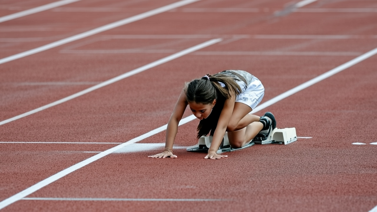
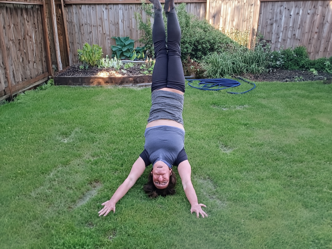
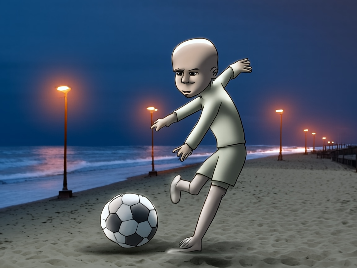
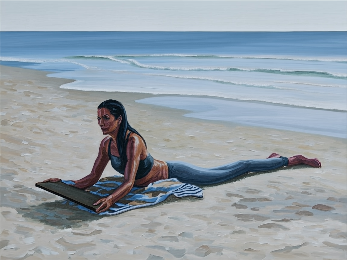
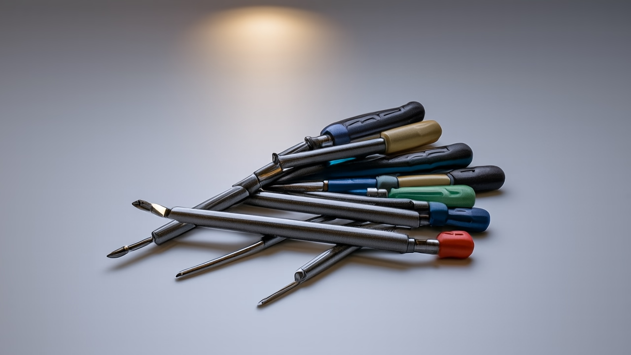
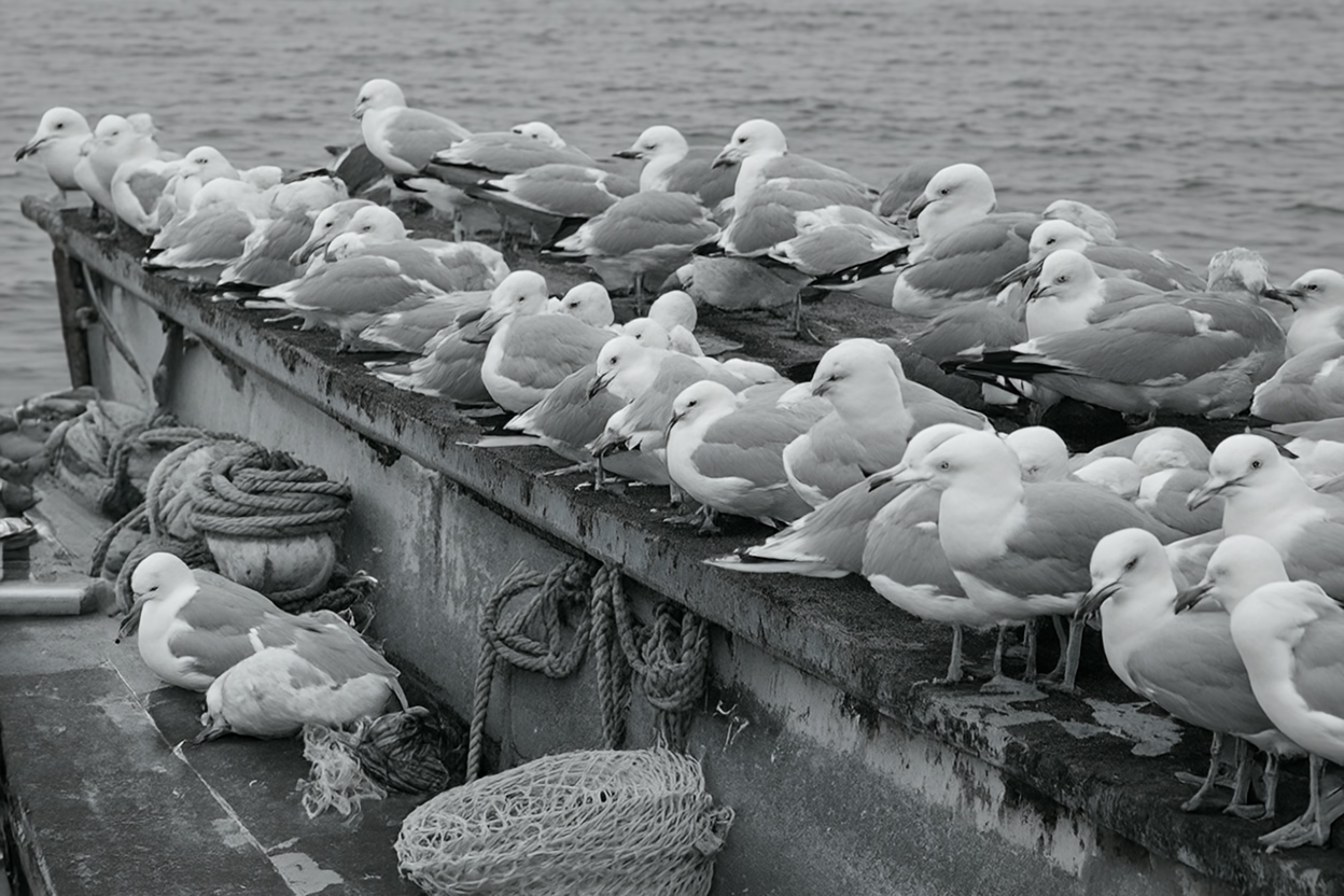
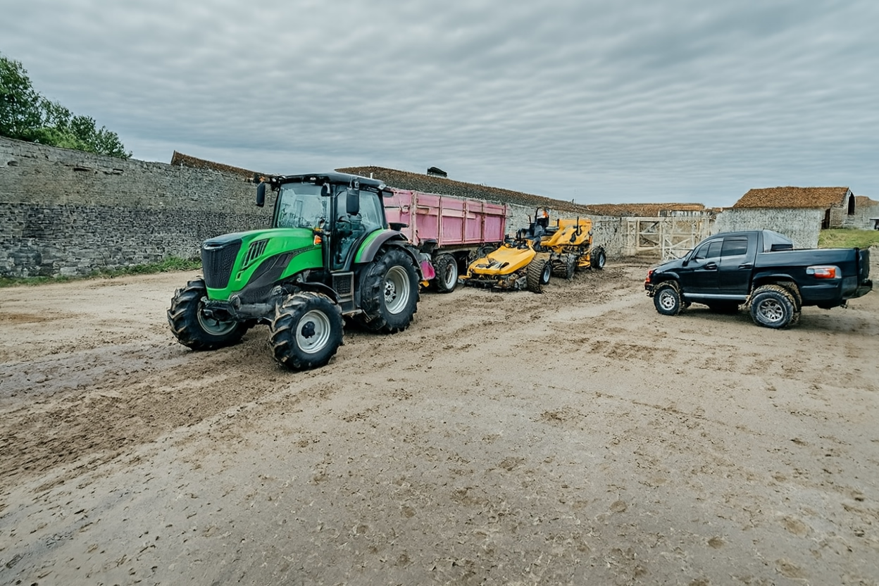
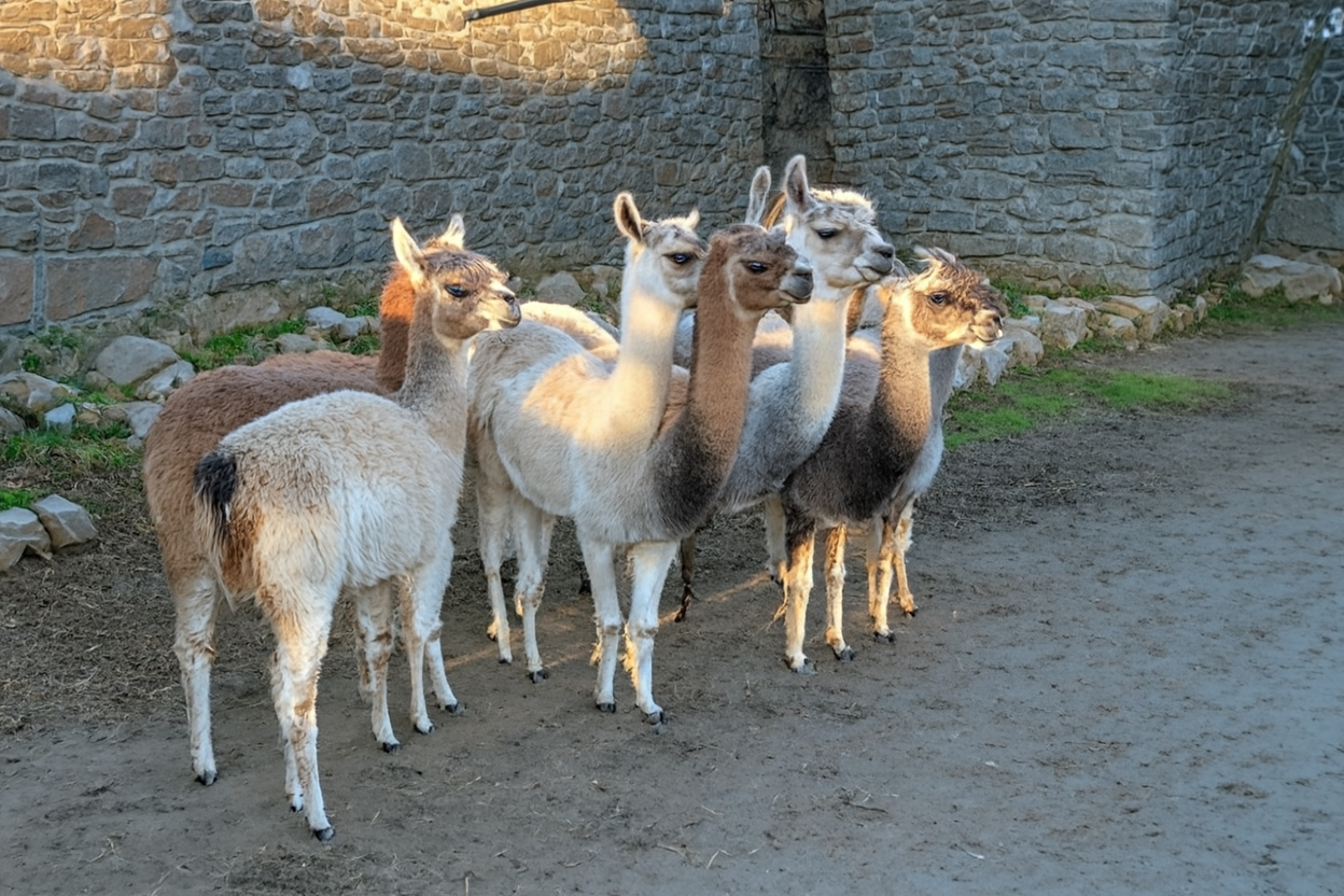
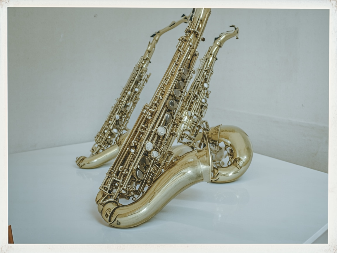
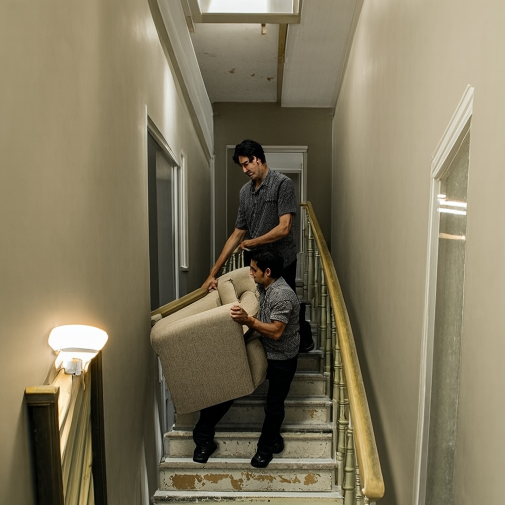
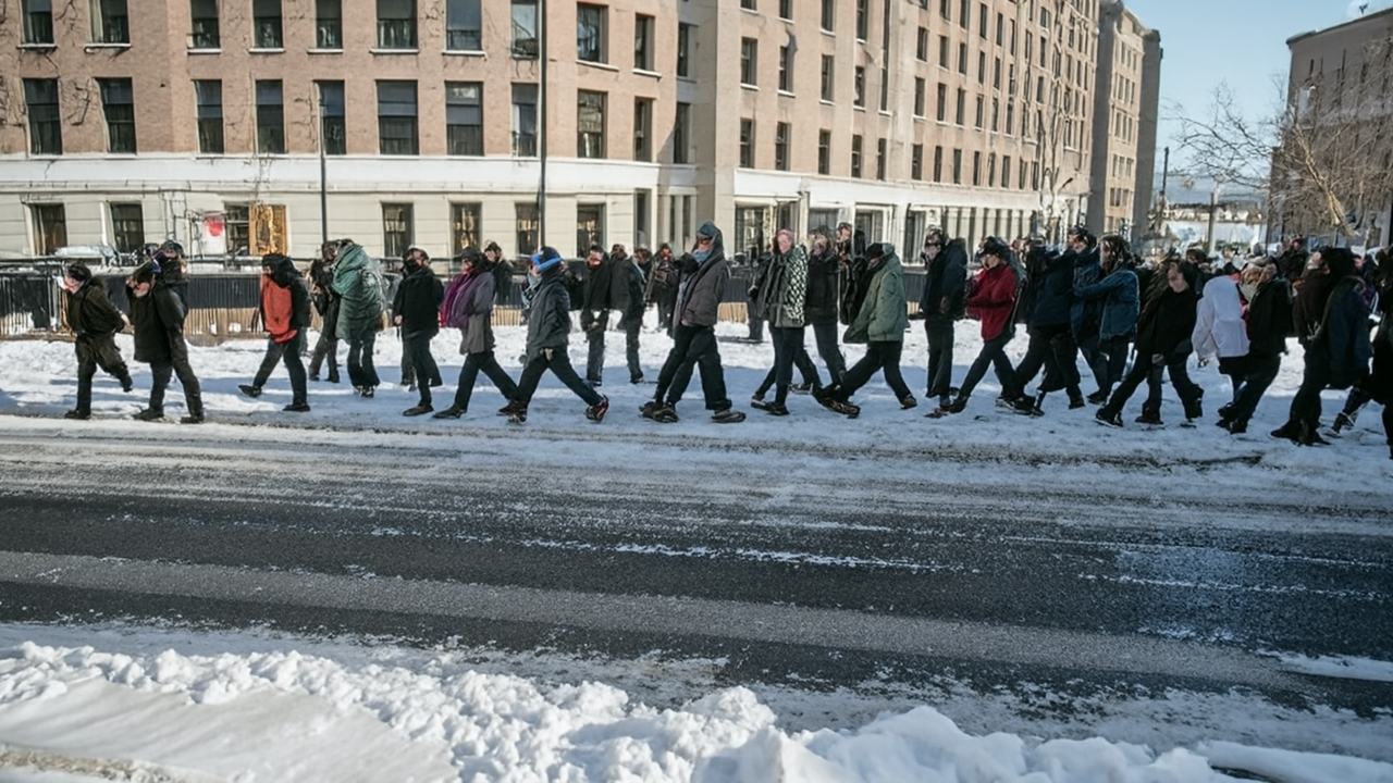
Full body: legs deformed on the starting blocks

Appendix A – Training Settings

training progress

phase 2 from 80M of 660M samples

share of training timesteps within 0.08 to 0.13 · hover the plot to move

phase 1 · LogitNormal(0.8, 0.8)

<0.05%

phase 2 · LogitNormal(−0.2, 1.0)

3.0%

phase 2 / phase 1

107×

Setting	512² stage	1024² stage
Samples	610.27M (297,985 steps)	49.97M (24,400 steps)
Global batch	2,048	2,048
Data	Images at native 512px-class sizes: 368×512, 512×512, 512×384, 512×336, 640×360	Images at native 1024px-class sizes: 864×1216, 1024×1024, 1152×864, 1248×832, 1280×720
Aspect-ratio mix	20% each, no resizing	20% each, no resizing
Noising		: the noise scale doubles with the side length
Timesteps	LogitNormal(0.8, 0.8) for the first 80M samples (step 39,063), then LogitNormal(−0.2, 1.0)	LogitNormal(−0.2, 1.0) throughout
Objective	x-prediction, v-loss, weight clamped at t = 0.1 · readouts at weight 1 · LPIPS 0.1 and P-DINO 0.01 on the final head for t ≤ 0.7 · PixelREPA 0.1
Optimizer	Muon (momentum 0.95, Nesterov) on the 2D block matrices · AdamW (β = 0.9, 0.999, ε = 1e-8) on the rest · Muon updates RMS-matched to AdamW
Learning rate	Peak 2e-4 · linear warmup over 1M samples · flat to 550M · 1 − √ decay to 2.5e-5 over the last 60M	Linear re-warm over 0.5M samples to 2.5e-5, then flat
Weight decay	0.1 (0 on biases)
Gradient clipping	1.0 (global norm)
EMA	Half-life 1,954 steps (4M samples), from 100M samples (step 48,829)	Half-life 977 steps (2M samples), from 2M samples
Spike-aware EMA	EMA updates pause for 250 steps when the gradient norm exceeds 10× its rolling median
Caption dropout	5%, for classifier-free guidance
Hardware	64× H100 (8 nodes) · bf16 · FSDP2 · 32 images per GPU	Same, as 4 accumulated microbatches of 8

For further details on the architecture and training losses, refer to the Appendix of P-JiT.

Authorship statement

We wrote all the words on this page. We used Claude Opus 5.5 to help us build the image gallery and diagrams.